Anti wind-up with prescribed-order anti wind-up filter and PI feedback controller

We show in this application how to use hinfstruct to design a PI feedback and a 2nd-order anti-windup (AW) block for a longitudinal rigid aircraft subject magnitude saturations on the control signal. The AW block is used to control the integrator load. In contrast to more conventional approaches, both components are computed simultaneously.

For details refer to J-M. Biannic and P. Apkarian, "Anti-windup design via nonsmooth multi-objective optimization", American Control Conference, San Francisco, 2011

Contents

Enter plant data

G = ss([-0.5 1; 0.8 -0.4],[-0.2;-5],eye(2), zeros(2,1) );
m = 1; p = 2;

Simulink diagram

Initialize controller blocks as dummies for linlft

s = tf('s') ;
Kalpha =1; Ki = 1; Kq = 1;
AW = rss(2,1,1);
stepVal = 40; deadZoneWidth = 20;

Build specifications

Enter reference model

s = tf('s');
Ref = (1/(s/4+1))^2; % reference model

Define specification channels using linlft

io = getlinio('AWsyn'); % w, r, alpha,  u , e
Blocks = {'AWsyn/Kalpha','AWsyn/Ki','AWsyn/Kq','AWsyn/AW'};

Build standard form for performance and robustness

Pperf = linlft('AWsyn',io([2 5]),Blocks);           % r -> e  perf
Probust = linlft('AWsyn',io([1 4 ; 2 5]),Blocks);   % (w,r) -> (u,e)  robust performance
Pu = linlft('AWsyn',io([2 4]),Blocks);              % penalize control signal
Psim = linlft('AWsyn',io([2 3]),Blocks);            % (w,r) -> (u,e)  simulation channels

Describe composite controller

Feedback controller as composite of PI and static gains

Kalpha = realp('Kalpha', 0) ;
Ki = realp('Ki', 0) ;
Kq = realp('Kq', 0) ;

Anti-windup block as 2nd-order state-space model

AW = ltiblock.ss('AW',2,1,1);

Define closed-loop objectives

CLperf = lft(Pperf, blkdiag(Kalpha , Ki , Kq , AW) ) ;     % nominal performance
CLrobust = lft(Probust, blkdiag(Kalpha , Ki , Kq , AW) ) ; % robust performance
CLu = lft(Pu, blkdiag(Kalpha , Ki , Kq , AW) ) ;           % realistic control

Add weighting and penalization and aggregate all specs.

W1 = 1/(s/2 + 1) ;
pen1 = 70;  pen2 = 0.01*pen1;

W2=(s+40*0.001)/(s/20+40);

H0 = blkdiag( pen1*W1*CLperf , pen2*blkdiag(1, W1)*CLrobust, W2*CLu  )  ;

Solve problem with hinfstruct

op = hinfstructOptions('RandomStart',2); % 2 restarts mean 3 initial points overall
[H,gam] = hinfstruct(H0,op) ; gam,

Final: Peak gain = 1.6, Iterations = 48
Final: Peak gain = 1.6, Iterations = 71
Final: Peak gain = 70, Iterations = 5
       Spectral abscissa -1.08e-07 is close to bound -1e-07

gam =

    1.6033

Recover static gains and dynamic AW blocks

Kalpha = H.Blocks.Kalpha.Value , Ki = H.Blocks.Ki.Value ,
Kq = H.Blocks.Kq.Value , AW = ss(H.Blocks.AW) ;
AWstore = AW; % store anti-windup block

Kalpha =

  -31.1447


Ki =

  -66.1159


Kq =

   -4.8392

Simulate without magnitude saturations (nominal case)

close all;
stepVal = 40 ; deadZoneWidth = Inf; figure;
sim('AWsyn');
figure(1); clf;
subplot(211); plot(alpha.time,alpha.signals.values, yRef.time, yRef.signals.values,'--') ; grid
legend('alpha','reference signal');
title(' simulation without magnitude saturations ');
subplot(212); plot(u.time,u.signals.values,'--', uSat.time, uSat.signals.values) ; grid
legend('control before saturation','saturated control');

Warning: Using a default value of 0.2 for maximum step size.  The simulation step size will be equal
to or less than this value.  You can disable this diagnostic by setting 'Automatic solver parameter
selection' diagnostic to 'none' in the Diagnostics page of the configuration parameters dialog 

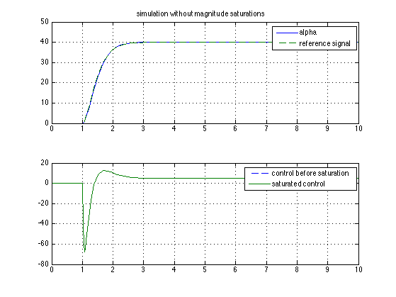
simulation without magnitude saturations

Simulate with magnitude saturations but without anti-windup (AW off)

stepVal = 40 ; deadZoneWidth = 20; figure;
AW = 0*AWstore;   % no AW
sim('AWsyn');
figure(2); clf;
subplot(211); plot(alpha.time,alpha.signals.values, yRef.time, yRef.signals.values,'--') ; grid
legend('alpha','reference signal');
title(' simulation with magnitude saturations and without AW ');
subplot(212); plot(u.time,u.signals.values,'--', uSat.time, uSat.signals.values) ; grid
legend('control before saturation','saturated control');

Warning: Using a default value of 0.2 for maximum step size.  The simulation step size will be equal
to or less than this value.  You can disable this diagnostic by setting 'Automatic solver parameter
selection' diagnostic to 'none' in the Diagnostics page of the configuration parameters dialog 

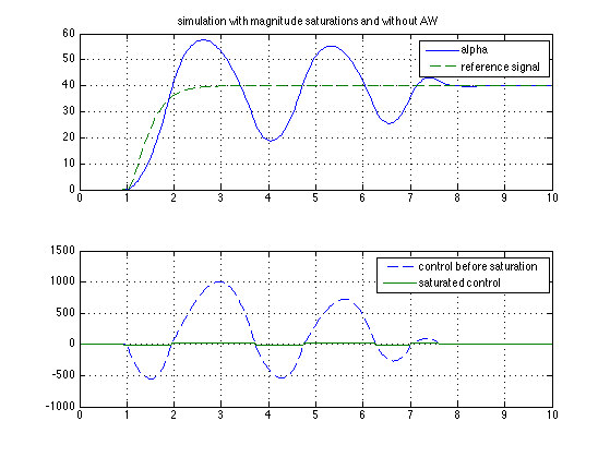
simulation with magnitude saturations and without AW

Simulate with magnitude saturations and anti-windup (AW on)

stepVal = 40 ; deadZoneWidth = 20; figure;
AW = AWstore ;  % with  AW
sim('AWsyn');
figure(3); clf;
subplot(211); plot(alpha.time,alpha.signals.values, yRef.time, yRef.signals.values,'--') ; grid
legend('alpha','reference signal');
title(' simulation with magnitude saturations and  AW ');
subplot(212); plot(u.time,u.signals.values,'--', uSat.time, uSat.signals.values) ; grid
legend('control before saturation','saturated control');

Warning: Using a default value of 0.2 for maximum step size.  The simulation step size will be equal
to or less than this value.  You can disable this diagnostic by setting 'Automatic solver parameter
selection' diagnostic to 'none' in the Diagnostics page of the configuration parameters dialog 

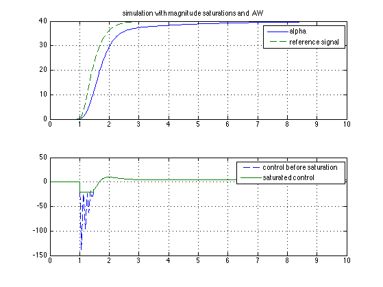
simulation with magnitude saturations and AW

Published with MATLAB® 7.12