Synthesis of decentralized PI controllers

We consider the design of a decentralized PI controller for the glass tube manufacturing plant described in "Tuning decentralized PID controllers for performance and robust stability", E. Kozakova, ICIC Express Letters, 2(2), 2008.

Plant data
Define decentralized 2x2 PI controller
Solve $H_\infty$ problem with hinfstruct
Show local PI controllers and retrieve decentralized controller C
Simulations and frequency-domain analysis

Plant data

load dataManufacturingPlant;

number of states

order(G),

ans =

     8

I/O sizes

iosize(G),

ans =

     2     2

Define decentralized 2x2 PI controller

C1 = ltiblock.pid('C1','pi');
C2 = ltiblock.pid('C2','pi');
C = blkdiag(C1,C2); % compound local PI controllers

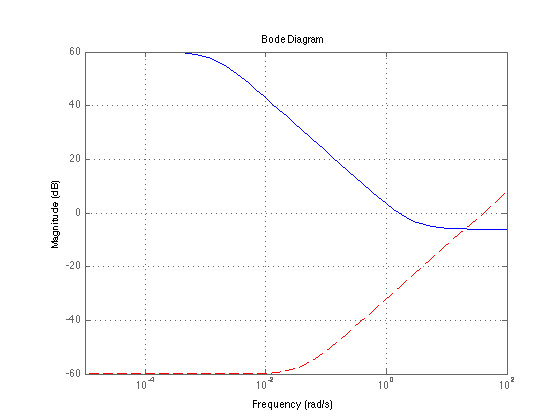
Now construct synthesis plant with appropriate weighting functions. Performance weight translates a minimum bandwidth of 1.4 rad/s and steady-state accuracy.

% performance weight
lfG=1e3;  % desired low frequency gain
hfG=0.5;  % desired high frequency gain
w0= 1.4 ; % desired crossover
wS=(hfG*s+w0)/(s+w0/lfG);

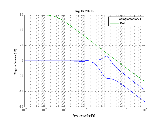
Robustness weight accounts for uncertainty/noise in the high-frequency range

lfG=0.001; % desired low frequency gain
hfG= 40;   % desired high frequency gain
w0=  40;   % desired crossover
wT=(s+w0*lfG)/(s/hfG+w0);
bodemag(wS,'b-',wT,'r--'); grid;
% Derive augmented plant
P = augw(G,wS*eye(2) ,[] , wT*eye(2) );

Form closed-loop interconnection

CL0 = lft(P,C);

Solve $H_\infty$ problem with `hinfstruct`

op = hinfstructOptions('RandomStart',3);
[CL, gam] = hinfstruct(CL0,op);

Final: Peak gain = 1.38, Iterations = 59
Final: Peak gain = 1.38, Iterations = 49
Final: Peak gain = 1.38, Iterations = 46
Final: Peak gain = 1.38, Iterations = 43

Note since gam > 1 the specified control structure fails to achieve performance requirements as expressed by the weighting functions.

Show local PI controllers and retrieve decentralized controller C

C1 = pid(CL.Blocks.C1),
C2 = pid(CL.Blocks.C2),
C = getNominal(C,CL);

Continuous-time PI controller in parallel form:
 
           1 
Kp + Ki * ---
           s 
 
With Kp = 0.0528, Ki = 0.0674
 
Continuous-time PI controller in parallel form:
 
           1 
Kp + Ki * ---
           s 
 
With Kp = 5.51, Ki = 3.5

Simulations and frequency-domain analysis

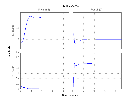
Perform simulations with set-point driven with 1/(s/8 + 1)

Tsim = (1/(s/8+1)*eye(2))*feedback(G*C,eye(2)) ;
step(Tsim); grid;

Show robustness constraints

sigma(feedback(G*C,eye(2)) , 1/wT); grid;
legend('complementary T', '1/wT');