Feed-forward & feedback synthesis with prescribed controller structures
This example illustrates the design of a conventional 2-DOF control structure with restricted complexity of components.
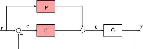
- The feedback component consists of a PID controller.
- The feed-forward block is a 2nd-order filter.
Contents
Define nominal plant
s = tf('s');
ny = 1; nu = 1;
G = ss( 1/(s-1) ); % unstable SISO plant
Build synthesis interconnection and define specifications using linlft
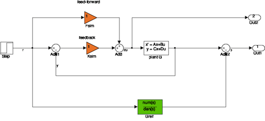
Define reference model capturing performance constraints.
num = 11.11; den = [1 6 11.11] ;
Gref = tf(num , den); % reference model
io = getlinio('TwoDOF'); % r, zu, e and y
Blocks = {'TwoDOF/Ksim','TwoDOF/Fsim'};

Pperf = linlft('TwoDOF',io([1 3]),Blocks);       % r -> e  perf
Pu    = linlft('TwoDOF',io([1 2]),Blocks);       % penalize control signal
Psim  = linlft('TwoDOF',io([1 4]),Blocks);       % simulation channel
Define controller blocks
K = ltiblock.pid('K','pid');      % PID feedback
F = ltiblock.ss('F',2, nu, ny );  % feed-forward of order 2
C0 = blkdiag(K,F);                % gather all blocks
Include weighting functions and aggregate objectives
W1 = (0.25*s+0.6)/(s+0.006); % performance in the low frequency range
Wu = 0.01 ;                  % control signal penalization
% Gather closed-loop objectives through diagonal augmentation
CL0 = blkdiag( W1*lft(Pperf, C0), Wu*lft(Pu,C0) ) ;
Run hinfstruct
[CL,gam] = hinfstruct(CL0);
Final: Peak gain = 0.0177, Iterations = 83
Retrieve feedback and feed-forward blocks in transfer function format
Kpid = pid(CL.Blocks.K), Ftf = tf(CL.Blocks.F),
Continuous-time PIDF controller in parallel form:

           1            s
Kp + Ki * --- + Kd * --------
           s          Tf*s+1

With Kp = 3.05, Ki = 2.8, Kd = 167, Tf = 2.03e+05


Transfer function:
-3.763 s^2 - 24.35 s - 56.19
----------------------------
   s^2 + 13.82 s + 22.81
Check results
norm( ss(CL) , inf), gam,
ans =

    0.0176


gam =

    0.0177
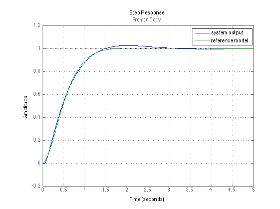
Simulate set-point responses
CLsim = lft(Psim, blkdiag(Kpid,Ftf) );
figure(8); clf; step(CLsim , 5); grid; hold on; step(Gref,5);
legend('system output', 'reference model') ;