Loop-shaping with a MIMO PID and a setpoint filter
hinfstruct is used to design a MIMO PID controller and a setpoint filter from a standard loop-shaping arrangement as defined by Glover & MacFarlane.
Example borrowed from Genc, A. U., A state-space algorithm for designing H-infinity loop-shaping PID controllers. Tech. report, Cambridge, UK: Cambridge University, 2000.
http://www-control.eng.cam.ac.uk/aug20/aug20.html
See also P. Apkarian, V. Bompart and D. Noll Nonsmooth Structured Control Design with Application to PID Loop-Shaping of a Process. International Journal of Robust and Nonlinear Control, vol. 17, no. 14, pp. 1320-1342, 2007.

Contents
- Plant description and design objectives
- Define MIMO PID and pre- and post-compensators
- Build loop-shaping synthesis interconnection
- Tune MIMO PID controller using hinfstruct
- Time-domain simulations of actual chemical process with feedback alone
- Reduce undesirable couplings and smoothen responses using a prefilter
Plant description and design objectives
We consider a 2x2 chemical process consisting of a 24-tray tower for separating methanol and water. The transfer matrix model for controlling the temperature on the 4th and 17th trays is given as:
% actual plant with delays
tf11 = -2.2*tf(1,[7 1]);     tf11.inputd = 1;
tf12 =  1.3*tf(1,[7 1]);     tf12.inputd = 0.3;
tf21 = -2.8*tf(1,[9.5 1]);   tf21.inputd = 1.8;
tf22 =  4.3*tf(1,[9.2 1]);   tf22.inputd = 0.35;
Gactual = [tf11 tf12;tf21 tf22];   % plant with exact delays
set(Gactual,'outputname',{'t17' 't4'});
set(Gactual,'inputname',{'u1' 'u2'});
For synthesis purpose delays are replaced with 2nd-order Padé approximations. This leads to a model of order 12.
[n,d]=  pade(1,2);   del11=tf(n,d);
[n,d]=  pade(0.3,2); del12=tf(n,d);
[n,d]=  pade(1.8,2); del21=tf(n,d);
[n,d]=  pade(0.35,2); del22=tf(n,d);
% plant rational approximation
G = [-2.2*del11*tf(1,[7 1]) 1.3*del12*tf(1,[7 1]); ...
     -2.8*del21*tf(1,[9.5 1]) 4.3*del22*tf(1,[9.2 1])];
set(G,'outputname',{'t17' 't4'});
set(G,'inputname',{'u1' 'u2'});
Design objectives include
- Settling times of about 10 seconds for setpoint responses t17 and t4
- Good decoupling between temperatures t17 and t4.
- Noise attenuation in the high frequency range.
- Good robustness margins as defined by MacFarlane and Glover (1990). Margins are relative to coprime factor uncertainties. In general, 25% uncertainty (H-infinity norm less than 4) is considered a good design.
Figures 1 and 2 are equivalent through the transformation

The loop-shaping interconnection of figure 2 is used to synthesize a MIMO PID controller. The overall controller is then finally obtained as

This is an composite of a MIMO PID and a roll-off filter W2 which has better noise attenuation than pure PID controllers.
Define MIMO PID and pre- and post-compensators
Pre- and post-compensators reflect desired loop shapes:
W1 = [tf([5 2],[1 0.001]) 0; ...
      0 tf([5 2],[1 0.001])];
W1i = 1/W1;
W2 = [tf(10,[1 10]) 0; 0 tf(10,[1 10])];

sigma(W1,W2,'r--'); grid; legend('W1 performance','W2 roll-off');
title('pre- and post-compensators');

Build loop-shaping synthesis interconnection
Describe MIMO PID controller
Kp = realp('Kp',zeros(2));
Ki = realp('Ki',zeros(2));
Kd = realp('Kd',zeros(2));
tau = realp('tau', 1);     % non-zero is realizable

Kpid = Kp + Ki*tf(1,[1 0]) + Kd*tf([1 0],[tau 1]) ;
Describe synthesis interconnection loop
W1.u = 'w1'; W1.y = 'y1';
G.y = 'y';
W2.u = 'y' ;  W2.y = 'y2';
Kpid.y = 'u';
Sum1 = sumblk('z1 = w2 + y2',2);
Sum2 = sumblk('s2 = y1 + u',2);
Kpid.u = 'z1';
G.u = 's2';
W1i.u = 'u' ; W1i.y = 'z2';

% connect blocks together
T0 = connect(G,Kpid,W1,W1i,W2,Sum1,Sum2,{'w1','w2'},{'z1','z2'});
Tune MIMO PID controller using hinfstruct
op = hinfstructOptions('RandomStart',3); % multiple restarts may improve
[T,gam] = hinfstruct(T0,op);
Final: Peak gain = 2.92, Iterations = 81
Final: Peak gain = 2.91, Iterations = 144
Final: Peak gain = 2.92, Iterations = 155
Final: Peak gain = 3.69, Iterations = 66
A value of
1/gam,
ans =

    0.3431
relative coprime factor uncertainty has been achieved
Display controller parameters
T.Blocks.Kp.Value, T.Blocks.Ki.Value,
T.Blocks.Kd.Value, T.Blocks.tau.Value,
% Retrieve MIMO PID controller
KpidFinal = getNominal(Kpid,T);
% Deduce final controller
Kfinal = KpidFinal*W2 ;
ans =

    2.5960   -0.7038
   -1.1410   -2.4019


ans =

    0.8455   -0.2434
    0.0461   -0.8983


ans =

    0.7437   -0.2777
   -1.5550    0.0193


ans =

    0.1523
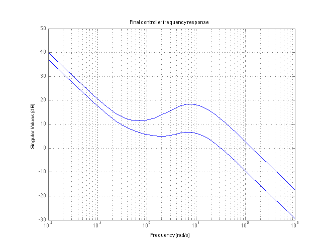
Display controller frequency response and check roll-off properties. Remind that controller is a composite of a MIMO PID and a roll-off filter W2.
figure(2); clf;
sigma(Kfinal); grid on; title('Final controller frequency response') ;
Time-domain simulations of actual chemical process with feedback alone
CLsim = feedback(Gactual*(-Kfinal),eye(2));
set(CLsim,'inputname',{'t17 setpoint' 't4 setpoint'});
figure(1); clf;
step(CLsim,30); grid;
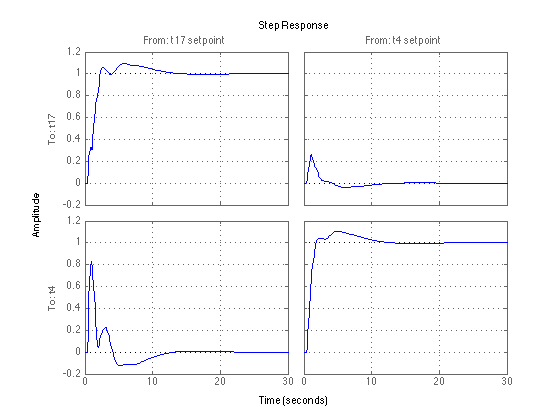
Unpleasant distorted responses are obtained along with strong couplings between t17 and t4. Using PID feedback alone is not sufficient in this application. A setpoint filter is therefore introduced to achieve better performance. Altogether, we end up with a 2-DOF control structure.
Reduce undesirable couplings and smoothen responses using a prefilter
A prefilter shapes setpoint inputs to enhance responses and reduce couplings between t17 and t4. Prefilter tuning can be based on a model reference tracking strategy. Note the feedback block is fixed which leaves unchanged robustness margins.
s = tf('s');
Gref = blkdiag(1/(3*s+1),1/(3*s+1) );  % reference model
Define setpoint filter with classical structure
tau1 = realp('tau1',1);
a1 = realp('a1',1); b1 = realp('b1',1); % realizability
tau2 = realp('tau2',1);
a2 = realp('a2',1); b2 = realp('b2',1); % realizability
F = [tf(1,[tau1 1])  tf([a1 0],[b1 1]);tf([a2 0],[b2 1]) tf(1,[tau2 1])] ;
Form synthesis problem as minimization of tracking error.
T0 = (feedback(G*(-Kfinal),eye(2))*F - Gref) ; % tracking error

% Tune setpoint filter
op = hinfstructOptions('RandomStart',3); % multiple restarts may improve
[T,gam] = hinfstruct(T0,op);
Ffinal = getNominal(F,T);
Final: Peak gain = 0.441, Iterations = 35
Final: Peak gain = 0.446, Iterations = 44
Final: Peak gain = 0.441, Iterations = 36
Final: Peak gain = 0.444, Iterations = 39
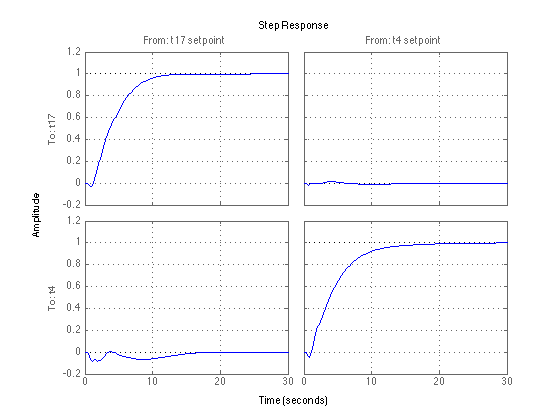
Time-domain simulations of actual chemical process with feedback and setpoint filter in place.
CLsim = feedback(Gactual*(-Kfinal),eye(2))*Ffinal;

set(CLsim,'inputname',{'t17 setpoint' 't4 setpoint'});
figure(3); clf;
step(CLsim,30); grid;