Tuning controllers for multiple models or operating conditions
Reliable or fault tolerant control refer to situations where the controlled plant may undergo deviations from its nominal mode of operation. Changes in operational mode may correspond to actuator or detector failures or abrupt changes in the dynamics due to various sources including model uncertainties. We show in this application that hinfstruct can cope with several operiational modes to increase safety of the controlled plant.
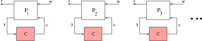
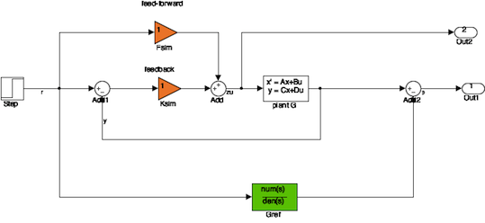
Problem borrowed from "A natural approach to high performance robust control: another look at the youla parameterization", K. Zhou, Proc. SICE 2004 pp. 869-874 We consider the synthesis of a 2-DOF control architecture for a family of models involving a nominal model G1 and 9 other models corresponding to faulty operational conditions or mismatch between the actual plant and the nominal model. The control architecture involves a PID feedback controller and a 2nd-order feed-forward block. The objective is to achieve good tracking properties as reflected by a reference model on the entire model family. Such problems are often referred to as multi-model or reliable or fault-tolerant control in the litterature.
Contents
- Define nominal model and faulty operational modes
- Build synthesis interconnection including reference model Gref
- Define controller blocks of 2-DOF control architecture
- Define and aggregate all tracking performance for all models
- Run hinfstruct with restarts
- Recover feedback and feed-forward blocks in transfer function format
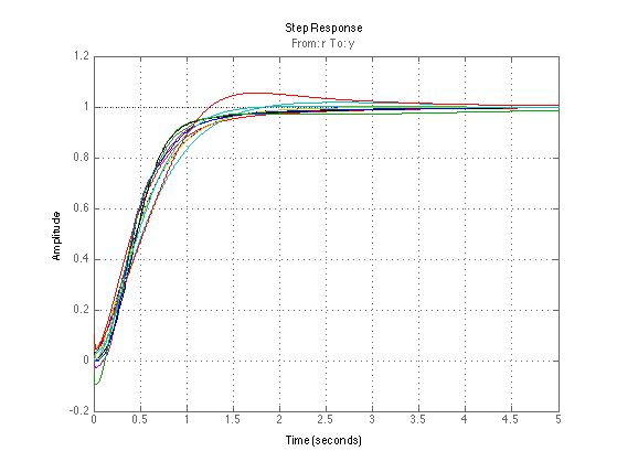
- Simulate set-point responses of all operational modes
Define nominal model and faulty operational modes
clear all;
s = tf('s') ; nu = 1; ny = 1;
Gmodel{1} = 1/(s-1) ; % nominal  plant
Gmodel{2} = 6.1/( (s-1)*(s+6.1) );
Gmodel{3} = 1.425/(s-1.425);
Gmodel{4} = 0.67/(s-0.67);
Gmodel{5} = (-0.07*s+1)/( (s-1)*(0.07*s+1) ) ;
Gmodel{6} = 70^2/( (s-1)*(s^2 +2*0.15*70*s+70^2) );
Gmodel{7} = 70^2/( (s-1)*(s^2+2*5.6*70*s+70^2) ) ;
Gmodel{8} = (1/(s-1))*( 50/(s+50) )^6 ;
Gmodel{9} = -2.9621*(s-9.837)*(s+0.76892)/( (s+32)*(s-1)*(s+0.56119) ) ;
Gmodel{10} = 4.991*(s^2+3.6722*s+34.848)/( (s+32)*(s+7.2408)*(s-1) ) ;
Build synthesis interconnection including reference model Gref
num = 11.11; den = [1 6 11.11] ;
Gref = tf(num , den); % reference model
G = ss(Gmodel{1});
io = getlinio('TwoDOF');                % r, zu, e and y  I/Os channels
Blocks = {'TwoDOF/Ksim','TwoDOF/Fsim'}; % sub-blocks to be optimized by |hinfstruct|
Define weighting functions
W1 = (0.25*s+0.6)/(s+0.006); % emphasize low frequency range for performance
Define controller blocks of 2-DOF control architecture
K = ltiblock.pid('K','pid');      % PID feedback
F = ltiblock.ss('F',2, nu, ny );  % feed-forward block of order 2
C0 = blkdiag(K,F);                % gather all blocks
Define and aggregate all tracking performance for all models
AllPerf = [];
for ii = 1:10
    G = ss(Gmodel{ii}) ;
    Pperf = linlft('TwoDOF',io([1 3]),Blocks);       % r -> e  perf
    Pu    = linlft('TwoDOF',io([1 2]),Blocks);       % penalize control signal
    AllPerf = blkdiag(AllPerf, W1*lft(Pperf , C0) );
end
CL0 = AllPerf ;
Run hinfstruct with restarts
op = hinfstructOptions('RandomStart',2,'Display','final');
[CL,gam] = hinfstruct(CL0, op);
Final: Failed to meet closed-loop stability constraint (spectral abscissa = 0.072)
Final: Peak gain = 0.0508, Iterations = 182
Final: Peak gain = 0.0631, Iterations = 157
Recover feedback and feed-forward blocks in transfer function format
Kpid = pid(CL.Blocks.K), Ftf = tf(CL.Blocks.F),
Continuous-time PIDF controller in parallel form:

           1            s
Kp + Ki * --- + Kd * --------
           s          Tf*s+1

With Kp = 6.54, Ki = 3.13, Kd = 0.467, Tf = 0.0994


Transfer function:
103.6 s^2 - 4.253e04 s - 6.77e04
--------------------------------
    s^2 + 4023 s + 2.457e04
Simulate set-point responses of all operational modes
figure(9); clf;
for ii = 1:10
  G = ss(Gmodel{ii}) ;
  Psim= linlft('TwoDOF',io([1 4]),Blocks);       % r -> y
  CLsim = lft(Psim, blkdiag(Kpid,Ftf) );
  step(CLsim , 5);  hold on;
end
step(Gref,5);  grid;
hold off;