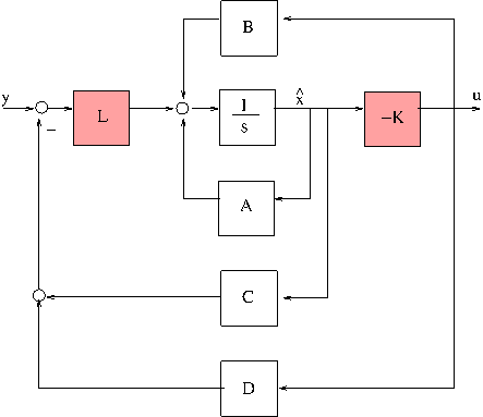
Observer-based controller
A streamlined fashion to define an observer-based controller and solve for it with hinfstruct. We consider the example of the Active Suspension Control from the Robust Control Toolbox, Control Design 1.
Contents
Define augmented plant:
nx = 6; ny = 1; nu = 1; nw = 2; nz = 2;
A =   [0   1.0000e+00            0            0            0            0 ;
  -5.5800e+01  -3.4483e+00   5.5800e+01   3.4483e+00            0            0;
            0            0            0   1.0000e+00            0            0;
   2.7427e+02   1.6949e+01  -3.4946e+03  -1.6949e+01            0            0;
            0            0            0            0  -5.0000e+02            0;
   1.6000e+01            0            0            0            0  -3.1416e+01];

B = [0            0            0;
     0            0   3.4483e+01;
                  0            0            0;
    2.2542e+02    0  -1.6949e+02;
            0     0   6.4000e+01;
            0     0            0];

C = [ 0            0            0            0  -5.4087e+01            0;
      0            0            0            0            0   1.5708e+01;
   1.0000e+00            0  -1.0000e+00      0            0            0];

D = [0      0   7.6923e+00;
     0            0            0;
     0   1.0000e-02            0];

P = ss(A,B,C,D);
Define observer-based controller.
P22 = P(nz+(1:ny),nw+(1:nu)) ;
[A,B,C,D] = ssdata(P22) ;          % u to y plant
K = realp('K',zeros(nu,nx));       % state feedback
L = realp('L',eye(nx,ny));         % observer gain
OBC = ss(A-B*K-L*(C-D*K),L,-K,0) ; % observer-based controller in state-space format
Define closed-loop interconnection
CL0 = lft(P,OBC);
Solve  problem with hinfstruct
[CL,gam1] = hinfstruct(CL0); % CL is tuned version of CL0
Final: Peak gain = 0.609, Iterations = 80
Get state feedback and observer gains
CL.BLocks.K.Value, CL.BLocks.L.Value,
ans =

   44.5934   15.6852 -114.5391    0.3011   -2.2210  -54.6811


ans =

   1.0e+03 *

    0.0206
    0.1825
   -0.0066
    0.5587
   -2.2661
    0.0270
Compare with hinfsyn (full-order black-box controller).
[K,clp,gam2] = hinfsyn(P,ny,nu) ;
% Output achieved objective.
fprintf(1,' Achieved H-infinity norms  HINFSTRUCT:%6.2f  HINFSYN:%6.2f \n\n', gam1,gam2);
Achieved H-infinity norms HINFSTRUCT: 0.61 HINFSYN: 0.61