Pole placement and decoupling with a MIMO PI controller
We show in this illustration how to use hinfstruct and eigenspace pole placement techniques to design a MIMO PI controller for a launcher in atmospheric flight. The synthesis is performed at iso dynamics, i.e., in the set of PI controllers assigning prescribed dynamics in closed loop.
Problem borrowed from "Eigenstructure versus optimal control for decoupling" by A.P. Oliva, W.C. Leite Filho, CEP 10, 2002.
Contents
State-space data and specs.
The state vector is defined as
- w: vertical velocity (m/s)
- q: pitch rate (deg./s)
- theta: pitch angle (deg.)
- v: lateral velocity (m/s)
- r: yaw rate (deg./s)
- psi: yaw angle (deg.)
- p: roll rate (deg./s)
- phi: roll angle (deg.)
with measurements y = ( q theta r psi p phi )
The control signal is defined as u = ( bz by br ) with
- bz control deflection of the pitch nozzle actuator (deg.)
- by control deflection of the yaw nozzle actuator (deg.)
- br control deflection of the roll nozzle actuator (deg.)
Performance specifications include
- decoupling of the 3 axes (theta, q), (psi, r), and (phi, p)
- well-damped responses to set-points in theta, psi and phi with settling times around 2.5 sec.
Since the controller parametrization ensures partial assignment of appropriate closed-loop dynamics, hinfstruct is used primarily to polish axis decoupling and to garantee stability of unassigned modes.
Construct launcher state-space data A, B, C and D
clear all; close all;
teta0=8.38; psi0=3.48; phi0=11.99;
Zw=-0.0162;ZqU0=87.9;Zteta=-9.48;Zv=0.0006;Zpsi=-2.013;Zp=-0.687;Zphi=0.399;
Mw=0.0022;Mq=0.0148;Mr=-0.0005;Mp=0.0042;Tq=0.98;Tr=-0.2084;Yw=-6e-4;Yteta=-2.11;
Yv=Zw;Yr=-ZqU0;Ypsi=9.47;Yp=-1.965;Yphi=1.3272;Nq=5e-4;Nv=-Mw;Nr=0.0151;Np=-0.0024;
Pq=0.2078;Pr=0.9782;Lq=0;Lr=0;Lp=-0.0289;Fq=0.0704;Fr=-0.015;Zbz= 10.87;Mbz= 4.08;
Yby=-10.87;Nby=4.08;Lbr=25.89;

nx = 8; nu = 3; ny = 6;
A=[Zw ZqU0 Zteta Zv 0 Zpsi Zp Zphi;Mw Mq 0 0 Mr 0 Mp 0;0 Tq 0 0 Tr 0 0 0; ...
    Yw 0 Yteta Yv Yr Ypsi Yp Yphi;0 Nq 0 Nv Nr 0 Np 0;0 Pq 0 0 Pr 0 0 0; ...
    0 Lq 0 0 Lr 0 Lp 0;0 Fq 0 0 Fr 0 1 0];
B=[Zbz Mbz 0 0 0 0 0 0;0 0 0 Yby Nby 0 0 0;0 0 0 0 0 0 Lbr 0]';

C = [0 1 0 0 0 0 0 0;0 0 1 0 0 0 0 0;0 0 0 0 1 0 0 0;
     0 0 0 0 0 1 0 0;0 0 0 0 0 0 1 0;0 0 0 0 0 0 0 1] ;

G = ss(A,B,C,0, ...
    'outputname',{'q' 'theta'  'r' 'psi' 'p' 'phi'}, ...
    'inputname',{'theta command' 'psi command'  'phi command'}); % launcher model
Add integrals of theta, psi and phi to the model for steady-state control and generate augmented plant.
Hx = [0 0 1 0 0 0 0 0;0 0 0 0 0 1 0 0;0 0 0 0 0 0 0 1];
Aa=[A zeros(8,3);Hx zeros(3) ]; Ba=[B;zeros(3)]; Ca = blkdiag(C , eye(3) ) ;
nxa = nx + 3 ;
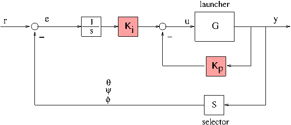
PI control architecture

PI control architecture
PI controller modal parametrization
Next we use eigenstructure assignment techniques to parametrize the set of MIMO PI controllers assigning prescribed dynamics in closed-loop. Note only partial pole placement is achieved since the full state vector is not accessible. Desired dynamics for the 3 axes (theta, q int theta), (psi, r, int psi), and (phi, p, int phi) are as follows.
% complex modes
ksi = sqrt(2)/2; % desired damping

om1 = 2.1;
lam1 = -om1*( ksi + 1i*sqrt(1-ksi^2) );
lam1conj = -om1*( ksi - 1i*sqrt(1-ksi^2) );

om2 = 2.2;
lam2 = -om2*( ksi + 1i*sqrt(1-ksi^2) );
lam2conj = -om2*( ksi - 1i*sqrt(1-ksi^2) );


om3 = 1.8;
lam3 = -om3*( ksi + 1i*sqrt(1-ksi^2) );
lam3conj = -om3*( ksi - 1i*sqrt(1-ksi^2) );

% real modes
om4 = 3.5 ;
lam4 = -om4;

om5 = 4 ;
lam5 = -om5;

om6 = 4.5 ;
lam6 = -om6;
Now parameterize static output feedback controllers assigning the prescribed spectrum using eigenspace degrees of freedom (so-called input vectors xi).
rng('default')
lam = lam1 ;
x1R=realp('x1R',randn(nu,1));
x1I=realp('x1I',randn(nu,1));
v1 =  (Aa-lam*eye(nxa))\(Ba*(x1R+1i*x1I)) ;
v1b = (Aa-conj(lam)*eye(nxa))\(Ba*(x1R-1i*x1I)) ;

lam = lam4 ;
x2=realp('x2',randn(nu,1));
v2 =  (Aa-lam*eye(nxa))\(Ba*x2) ;

lam = lam2 ;
x3R=realp('x3R',randn(nu,1));
x3I=realp('x3I',randn(nu,1));
v3 =  (Aa-lam*eye(nxa))\(Ba*(x3R+1i*x3I)) ;
v3b = (Aa-conj(lam)*eye(nxa))\(Ba*(x3R-1i*x3I)) ;

lam = lam5;
x4=realp('x4',randn(nu,1));
v4 =  (Aa-lam*eye(nxa))\(Ba*x4) ;


lam = lam3 ;
x5R=realp('x5R',randn(nu,1));
x5I=realp('x5I',randn(nu,1));
v5 =  (Aa-lam*eye(nxa))\(Ba*(x5R+1i*x5I)) ;
v5b = (Aa-conj(lam)*eye(nxa))\(Ba*(x5R-1i*x5I)) ;

lam = lam6 ;
x6=realp('x6',randn(nu,1));
v6 =  (Aa-lam*eye(nxa))\(Ba*x6) ;


X = [x1R+1i*x1I x1R-1i*x1I x2 x3R+1i*x3I x3R-1i*x3I x4 x5R+1i*x5I x5R-1i*x5I x6] ;
V = [v1 v1b v2 v3 v3b v4 v5 v5b v6] ; % eigenvectors
% finalize parametrization
Ka = X/(Ca*V) ;    % augmented static output feedback controller gathering PI blocks
Check closed-loop dynamics with parameterized (initial) controller
KaInit = real( getNominal(Ka) );  % clean out imaginary residues
eig(Aa-Ba*KaInit*Ca), % negative feedback
ans =

  -4.5000e+00
  -4.0000e+00
  -3.5000e+00
  -1.5556e+00 + 1.5556e+00i
  -1.5556e+00 - 1.5556e+00i
  -1.4849e+00 + 1.4849e+00i
  -1.4849e+00 - 1.4849e+00i
  -1.2728e+00 + 1.2728e+00i
  -1.2728e+00 - 1.2728e+00i
  -2.1974e-02 + 5.2786e-04i
  -2.1974e-02 - 5.2786e-04i
Define performance and simulation channels using linlft
% linearization I/Os
io = getlinio('launcherPI'); % r, e (theta, psi, phi),   y
Blocks = {'launcherPI/Kp','launcherPI/Ki'};

% build standard forms for tracking performance and simulation
Pperf = linlft('launcherPI',io([1 2]),Blocks);    % r -> e  perf
Psim  = linlft('launcherPI',io([1 4]),Blocks);    % r -> y  simulation channel
Show simulations of initial controller
Kp = KaInit(:,1:6); Ki = KaInit(:,7:9) ;  % separate proportional and integral MIMO gains
CLsim = lft(Psim , blkdiag(Kp,Ki) );      % close loop for simulation
set(CLsim,'outputname',{'q' 'theta'  'r' 'psi' 'p' 'phi'});
set(CLsim,'inputname',{'theta command' 'psi command'  'phi command'});
figure(4); clf; step(CLsim,10,'g--'); grid on;
title(' initial controller ');
pos = get(gcf,'Position'); set(gcf,'Position',[pos(1) pos(2) pos(3) 1.4*pos(3)]);

initial controller
Improve decoupling using hinfstruct
We observe strongly coupled responses for theta and psi set-point responses with the initial controller. Couplings are now reduced by minimizing the tracking error with hinfstruct. Also, since some residual poles are not assigned, hinfstruct is used to ensure internal stability of the closed-loop system.
Kp = Ka(:,1:6); Ki = Ka(:,7:9) ;     % separate proportional and integral MIMO gains
CL0 = lft(Pperf, blkdiag(Kp,Ki) );   % form tracking objective
[CL,gam] = hinfstruct(CL0) ;         % run solver

% Check closed-loop dynamics
eig(CL),
Final: Peak gain = 1.41, Iterations = 30

ans =

  -4.5000e+00 - 2.4275e-14i
  -4.0000e+00 - 5.0936e-15i
  -3.5000e+00 + 2.7599e-14i
  -1.5556e+00 - 1.5556e+00i
  -1.4849e+00 - 1.4849e+00i
  -1.2728e+00 - 1.2728e+00i
  -1.5556e+00 + 1.5556e+00i
  -1.4849e+00 + 1.4849e+00i
  -1.2728e+00 + 1.2728e+00i
  -2.2023e-02 - 5.9916e-04i
  -2.2023e-02 + 5.9916e-04i
Show simulations of final controller and observe how decouplings and been improved with respect to the initial controller.
% Get PI controller blocks and perform simulation
KpFinal = real( getNominal(Kp, CL) ); KiFinal = real( getNominal(Ki, CL) );
CLsim = lft(Psim , blkdiag(KpFinal,KiFinal) ) ;
set(CLsim,'outputname',{'q' 'theta'  'r' 'psi' 'p' 'phi'});
set(CLsim,'inputname',{'theta command' 'psi command'  'phi command'});


figure(5); clf;
step(CLsim,10,'b-'); grid on;
title(' final controller ');
pos = get(gcf,'Position'); set(gcf,'Position',[pos(1) pos(2) pos(3) 1.4*pos(3)]);

final controller
Observe decouplings, settling-times and overshoots meet specifications.