Reduced-order $H_\infty$ filtering

$H_\infty$ filtering viewed as a control problem can be solved using hinfstruct We consider a resonnant 2nd-order system with natural frequency 11 rad/s and damping ratio 0.1. The position y is corrupted by noise and the objective is to estimate the velocity signal z.

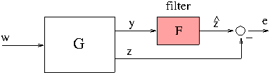
Enter plant with outputs y (measurements) and z (to be estimated)

G = ss([0 11;-11 -2.2],[0 0;1 0],[0 1;1 0],[0 1; 0 0]) ;

Define 2nd-order filter

F = ltiblock.ss('F',2,1,1);

Define $H_\infty$ index of the estimation error

CL0 = [F -1]*G ;

Solve $H_\infty$ filtering problem with hinfstruct with default + 3 restarts

op = hinfstructOptions('RandomStart',3,'Display','final');
[CL2nd,gam] = hinfstruct(CL0,op); %#ok<NASGU>

Final: Peak gain = 0.416, Iterations = 34
Final: Peak gain = 0.416, Iterations = 19
Final: Peak gain = 0.416, Iterations = 29
Final: Peak gain = 0.416, Iterations = 20

Get filter state-space data and transfer function

F2ss = ss(CL2nd.Blocks.F), tf(CL2nd.Blocks.F),

 
a = 
           F.x1    F.x2
   F.x1   1.067   5.441
   F.x2  -12.73  -3.322
 
b = 
              u1
   F.x1   -1.032
   F.x2  0.06803
 
c = 
          F.x1     F.x2
   y1  -0.9404  -0.1407
 
d = 
             u1
   y1  -0.06029
 
Continuous-time model.
 
Transfer function:
-0.06029 s^2 + 0.8252 s - 2.923
-------------------------------
     s^2 + 2.255 s + 65.71

Now synthesize a 1st-order filter

F = ltiblock.ss('F',1,1,1);
CL0 = [F -1]*G ;
op = hinfstructOptions('RandomStart',3,'Display','final');
[CL1st,gam] = hinfstruct(CL0,op); %#ok<NASGU>
F1ss = ss(CL1st.Blocks.F), tf(CL1st.Blocks.F),

Final: Peak gain = 0.416, Iterations = 31
Final: Peak gain = 0.416, Iterations = 20
Final: Peak gain = 0.416, Iterations = 16
Final: Peak gain = 0.416, Iterations = 22
 
a = 
           F.x1
   F.x1  -4.852
 
b = 
             u1
   F.x1  0.9256
 
c = 
        F.x1
   y1  2.411
 
d = 
             u1
   y1  -0.07645
 
Continuous-time model.
 
Transfer function:
-0.07645 s + 1.861
------------------
    s + 4.852

Plot error dynamics for both filters

opsigma = sigmaoptions; opsigma.MagUnits = 'abs';
sigmaplot(ss(CL2nd),'b',ss(CL1st),'g--',opsigma); grid;
legend('2nd-order  filter', '1st-order filter');

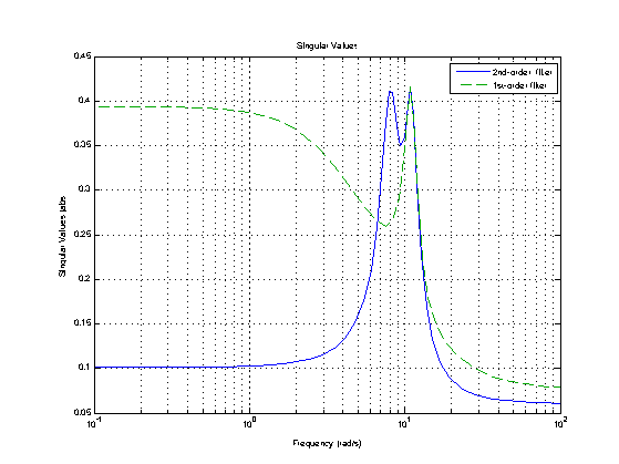
error dynamics for 2nd- and 1st-order filters

Reduced-order filtering

Reduced-order $H_\infty$ filtering