Benefits of direct synthesis of reduced-order controllers
We investigate full-order controller reduction and direct reduced-order synthesis with hinfstruct for the longitudinal axis control of the AIRC aircraft. The application demonstrates that synthesizing simpler controllers with hinfstruct may be a valid alternative when significant reduction of full-order  controllers is not possible.

Contents
- Problem description
- AIRC state-space data
- Define weighting functions for the sensitivity functions S, KS and T.
- Synthesize full-order controller with LMI technique
- Reduced full-order controller
- Run hinfstruct to synthesize reduced-order controller
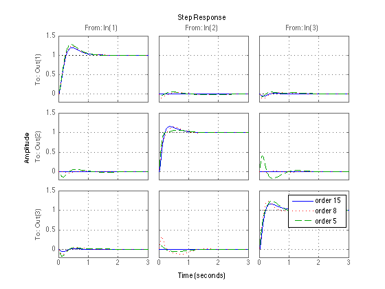
- Check controller performance through step responses in H, V and theta.
- Check roll-off properties.
- Analysis of pole-zero cancellations
AIRC aircraft control problem borrowed from "Multivariable feedback design", Addison-Wesley, Wokingham, UK. Maciejowski, J.M., 1989.
Problem description
The state vector is described as
- H: altitude (m)
- V: forward speed (m/s)
- theta: pitch angle (deg.)
- q: pitch rate (deg./s)
- Vz: vertical speed (m/s)
with control inputs
- u1: spoiler angle (tenth of degrees)
- u2: forward acceleration (m/s^-2)
- u3 elevator angle (deg.).
The measurements are H, V and theta.
The control objectives include
- A closed-loop bandwidth of about 10 rad/s
- Integral action in each loop for steady-accuracy
- Well-damped responses in H, V and theta with minimal overshoot
AIRC state-space data
load dataAIRC ;
Define weighting functions for the sensitivity functions S, KS and T.
s = tf('s');
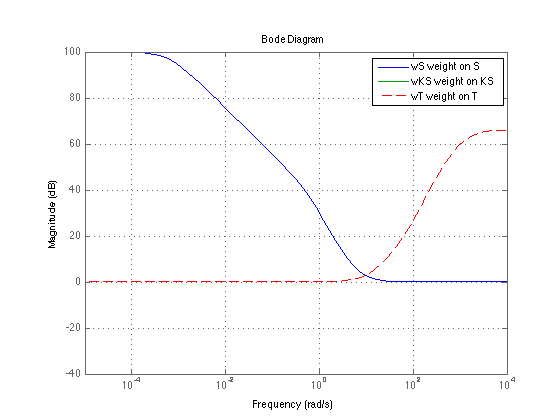
wS = (s+6)^2/( (s+0.0006)*(s+0.6) );  % tracking objectives
wKS = 0.01;                           % penalization on control signal
wT = 2000*(s+10)*(s+50)/(s+1000)^2 ;  % noise attenuation
Plot weighting functions
bodemag(wS,'-',ss(wKS),'g-',wT,'r--'); grid;
legend('wS weight on S','wKS weight on KS','wT weight on T');
% Form augmented plant and display problem dimensions.
P = augw(G,wS*eye(ny),wKS*eye(nu),wT*eye(ny) ); %
size(P),
State-space model with 12 outputs, 6 inputs, and 17 states.
Synthesize full-order controller with LMI technique
[K,CLlmi,gamLMI,INFO] = hinfsyn(P,ny,nu,'method','lmi')  ;
% Display controller order and $H_\infty$ performance
size(K, 'order'), gamLMI,
ans =

    17


gamLMI =

   2.5979e+00
Reduced full-order controller
Analysis of Hankel singular values suggests reducing the full-order controller to order 14.
hankelsv(K,'ncf','log');v=axis;
hold on; plot(v(1:2), ncfmargin(G,K)*[1 1],'--'); hold off;
K14=reduce(K,14,'errortype','ncf');
norm( lft(P, K14) , inf )
ans =

   3.6424e+02
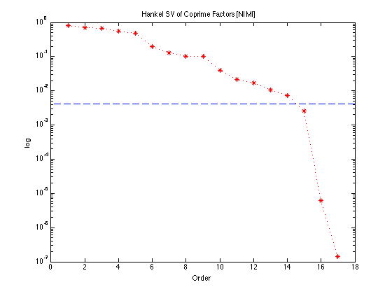
Reduction to order 14 is clearly not satisfactory since an -norm value close to 2.60 is expected. The full-order controller is thus reduced to order 15 without significant deterioration of performance.
K15=reduce(K,15,'errortype','ncf');
norm( lft(P, K15) , inf )
ans =

   2.6003e+00
Run hinfstruct to synthesize reduced-order controller
Consider now using hinfstruct to synthesize a reduced-order controller
k = 8;                                  % prescribed order
C  = ltiblock.ss('C',k,nu,ny);          % controller in state-space format
CL0 = lft(P , C);
[CL, gam] = hinfstruct(CL0);
C8 = ss( CL.Blocks.C  );                % store order 8 controller
norm( lft(P,C8), inf) ,
Final: Peak gain = 2.71, Iterations = 300

ans =

   2.7124e+00
A reduced-order controller of order 8 is already acceptable. If attempting to reduce further, trial-and-error indicates an order 5 may be acceptable.
k = 5;                                  % prescribed order
C  = ltiblock.ss('C',k,nu,ny);          % controller in state-space format
CL0 = lft(P , C);
op = hinfstructOptions('RandomStart',3,'MaxIter',400); % require higher accuracy
[CL, gam] = hinfstruct(CL0, op );

C5 = ss( CL.Blocks.C  );                % store order 5 controller
norm( lft(P,C5), inf) ,
Final: Peak gain = 2.92, Iterations = 400
Final: Peak gain = 2.92, Iterations = 400
Final: Peak gain = 3.29, Iterations = 400
Final: Peak gain = 3.22, Iterations = 400

ans =

   2.9158e+00
Check controller performance through step responses in H, V and theta.
T15 = feedback(G*K15,eye(ny));
T8 = feedback(G*C8,eye(ny));
T5 = feedback(G*C5,eye(ny));

step(T15,'b-', T8,'r:', T5,'g--', 3) ; grid;
legend('order 15','order 8','order 5') ;
Check roll-off properties.
Analysis indicates all controllers violate roll-off constraint.
sigma(T15,'b-', T8,'r:', T5,'g--',1/wT,'r') ; grid;
legend('order 15','order 8','order 5','1/wT') ;
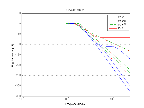
As expected, the higher-order controller provides better roll-off in the high-frequency range while C8 and C5 achieve better rise and settling times.
Analysis of pole-zero cancellations
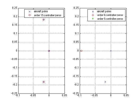
Examination of pole-zero cancellations shows that even reduced the controller of order 15 is critically sensitive to small variations in the plant data, an issue which is not present with C8 and C5 controllers.
subplot(121);
plot(pole(G),'bx'); hold on;
plot(zero(K15),'ro');
axis([-.1 0.05 -0.25 0.25]); grid on;
legend('aircraft poles','order 15 controller zeros');
hold off;
subplot(122);
plot(pole(G),'bx'); hold on;
plot(zero(C8),zeros(8,1),'ro'); hold on;       % zeros all real
plot(zero(C5),'gp'); hold on;
axis([-.1 0.05 -0.25 0.25]); grid on;
legend('aircraft poles','order 8 controller zeros','order 5 controller zeros');
hold off;
Warning: Imaginary parts of complex X and/or Y arguments ignored