Complex mu synthesis with reduced-order controller and D-scales

In this application, we address the synthesis of a robust controller for a plant subject to structured complex uncertainties. This is the called complex $\mu$ problem. Using hinfstruct, the design task is accomplished in one shot, that is, both controller and D-scales are obtained simultaneously.

We refer the reader to

P. Apkarian
Nonsmooth μ synthesis
Int. Journal of Robust and Nonlinear Control, 2011.

for $\mu$ synthesis problems involving abstract controller structures.

This illustration adresses the benchmark problem introduced in "Robust control of ill-conditioned plants, high purity distillation" IEEE Trans. Aut. Contr., 33(12), pp. 1092-1105, 1988. It consists of a distillation column where the overhead composition is to be controlled at yD = 0.99 and the bottom composition at xB = 0.01 both measured using the reflux L and the boilup V as control inputs.

Plant data
Define weightings
Describe controller
Build synthesis interconnection
Include static D-scales
Run hinfstruct
Validations

Plant data

An idealized linear model of the distillation column is obtained as follows:

load dataDistillColumn ;
G,

 
Transfer function from input 1 to output...
        87.8
 #1:  --------
      75 s + 1
 
       108.2
 #2:  --------
      75 s + 1
 
Transfer function from input 2 to output...
       -86.4
 #1:  --------
      75 s + 1
 
       -109.6
 #2:  --------
      75 s + 1

Define weightings

The uncertainty at the plant inputs are represented as relative multiplicative uncertainties leading to the plant family $G = G_0 (I+\Delta W_1(s))$ with $\bar \sigma(\Delta) \leq 1$ , where $W_1 = w_1 I_2$ with $w_1 = (s+0.2)/(0.5s+1)$ which gives the magnitude of the relative uncertainty in each input channel.

w1=0.2*(5*s+1)/(0.5*s+1); W1 = w1*eye(nu);
w1.TimeUnit = 'minutes';
figure; bodemag(w1); grid; legend('magnitude of w1');

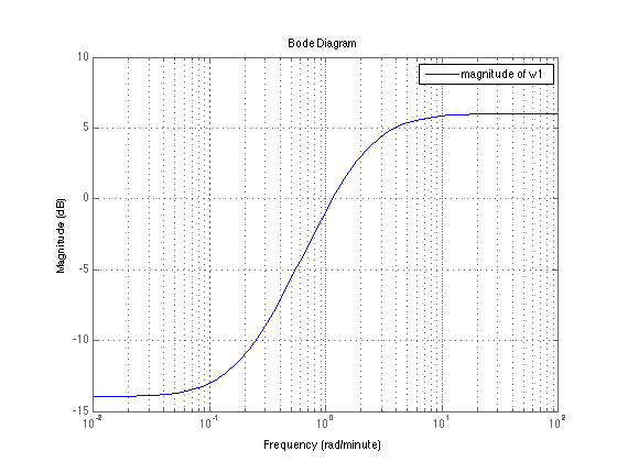
Note the uncertainty $\Delta$ has a 2x2 diagonal structure with 2 scalar blocks.

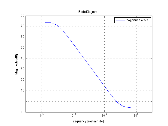
Performance is reflected through a weighting $W_p = w_p I_2$ of the sensitivity function S where $w_p = 0.5*(10*s+1)/10*s$ which empahsizes the need for integral action.

wp=0.5*(10*s+1)/(10*s+1e-4); Wp = wp*eye(ny);
wp.TimeUnit = 'minutes';
figure; bodemag(wp); grid; legend('magnitude of wp ');

Describe controller

The controller is sought as a 7th-order state model

C = ltiblock.ss('C',7,2,2);

Build synthesis interconnection

Now describes block interconnections using connect

C.y = 'u'; Sum1 = sumblk('s1 = u + di',2);
G.u = 's1'; G.y = 'yG'; Sum2 = sumblk('s2 = yG + do',2);
Sum3 = sumblk('s3 = -yG - do',2); C.u = 's3' ;
W1.u = 'u'; W1.y = 'uf';
Wp.u = 's2'; Wp.y ='yf';
% Connect the blocks together
T0 = connect(G,W1,Wp,C,Sum1,Sum2,Sum3,{'di','do'},{'uf','yf'});

Include static D-scales

The problem under consideration is a robust performance problem involving structured dynamic uncertainties and should be handled using a complex mu formulation. D-scales are thus introduced to capture uncertainty structure.

nxD = 3; % D-scale order for both uncertainty channels
D1 = ltiblock.tf('D1', nxD, nxD );
D2 = ltiblock.tf('D2', nxD, nxD );
% Aggregate D-scales with performance D-scale.
% Performance D-scale is set to identity.
D3 = ltiblock.gain('D3', zeros(2) ); D3.Gain.Free = false ;
D = blkdiag(D1, D2, D3);
% Now form overall synthesis interconnection with both controller
% blocks and D-scales.
T0 = (eye(4)-D)\T0*(eye(4)-D) ;

Run `hinfstruct`

[T,gam] = hinfstruct(T0); % multiple restarts may improve
% Get controller in state-space format
Css = ss(T.Blocks.C);

Final: Peak gain = 1.04, Iterations = 300

Validations

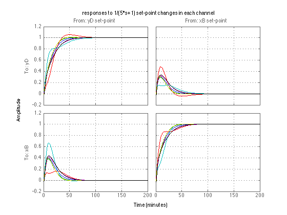
Validate controller on nominal and perturbed plants in the time domain with a set-point change driven by $1/(5s+1)$ .

figure
% nominal
Tsim = (1/(5*s+1)*eye(nu))*feedback(G*Css,eye(2));
Tsim.TimeUnit = 'minutes';
set(Tsim,'outputname',{'yD' 'xB'});
set(Tsim,'inputname',{'yD set-point' 'xB set-point '});
step(Tsim,200); hold on;

% 20% input gain variations
E = blkdiag(1.2,1.2);
Tsim = (1/(5*s+1)*eye(nu))*feedback(G*E*Css,eye(2));
Tsim.TimeUnit = 'minutes';
set(Tsim,'outputname',{'yD' 'xB'});
set(Tsim,'inputname',{'yD set-point' 'xB set-point '});
step(Tsim,200); hold on;

E = blkdiag(0.8,1.2);
Tsim = (1/(5*s+1)*eye(nu))*feedback(G*E*Css,eye(2));
Tsim.TimeUnit = 'minutes';
set(Tsim,'outputname',{'yD' 'xB'});
set(Tsim,'inputname',{'yD set-point' 'xB set-point '});
step(Tsim,200); hold on;

E = blkdiag(1.2,0.8);
Tsim = (1/(5*s+1)*eye(nu))*feedback(G*E*Css,eye(2));
Tsim.TimeUnit = 'minutes';
set(Tsim,'outputname',{'yD' 'xB'});
set(Tsim,'inputname',{'yD set-point' 'xB set-point '});
step(Tsim,200); hold on;

E = blkdiag(0.8,0.8);
Tsim = (1/(5*s+1)*eye(nu))*feedback(G*E*Css,eye(2));
Tsim.TimeUnit = 'minutes';
set(Tsim,'outputname',{'yD' 'xB'});
set(Tsim,'inputname',{'yD set-point' 'xB set-point '});
step(Tsim,200); hold on;
% Frequency-dependent distorsions in the input channels
f1 = 1-(s-0.2)/(0.5*s+1);
f2 = 1-(s+0.2)/(0.5*s+1);

E = blkdiag(f1,f1);
Tsim = (1/(5*s+1)*eye(nu))*feedback(G*E*Css,eye(2));
Tsim.TimeUnit = 'minutes';
set(Tsim,'outputname',{'yD' 'xB'});
set(Tsim,'inputname',{'yD set-point' 'xB set-point '});
step(Tsim,200); hold on;

E = blkdiag(f2,f2);
Tsim = (1/(5*s+1)*eye(nu))*feedback(G*E*Css,eye(2));
Tsim.TimeUnit = 'minutes';
set(Tsim,'outputname',{'yD' 'xB'});
set(Tsim,'inputname',{'yD set-point' 'xB set-point '});
step(Tsim,200); hold on; grid;
title(' responses to 1/(5*s+1) set-point changes in each channel');
hold off;